
I had always some loose thought in my mind which I’m eager but not able to systemically answer, which is what problem could/couldn’t be well solved by model machine learning/deep learning etc methodologies. In particular, I want to claim (loosely) that even if one can find the most powerful machine learning, it won’t be useful in predicting the financial or economics behavior in the world because it’s essentially ruled by game theory/mean field game theory, i.e., the outcome of the result really depends on the other players in the game so that no model could ‘predict’ it.
Admittedly, one can always give some frameworks to claim the effectiveness of ML in financial world, however, I’m eager to see very simple naive models to formalize this problem (either support or against my claim) in an elegant way.
 ) under the random splitting (this can be proved below). Next, when new test data is introduced, the reason we’re able to use such a data is based on the assumption that data distribution under the given won’t change.
  , as one can see that the essence of this model’s prediction power comes from the invariant quantity
  , it has prediction power only if
  matrix
 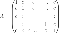 ?
? , where
  are identity and ones matrix respectively. Assume
  is an eigen-vector associated with an eigen-value
  , then
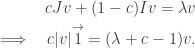
 , when
 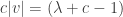 , i.e.,
  .
. when
when  , this is a
  dimension subspace
  .
. , where
  is an invertible matrix,
  .
. , and
, and  , we can solve the eigenvalue from the corresponding polynomial
 .
. .
. as event that the car is behind the door i,
  as event of your first guess,
  as event that the host opened the door i with a goat behind. Hence,
 . Therefore, the correct choice is to switch your decision from door 1 to door 2.
 , then
 is a big number, therefore, we’re not able to reject
  . Vice Versa for H_a.
 is a RKHS if
 ![|\mathcal{F}_t[f]|=|f(t)|\leq M\|f\|_{\mathcal{H}}, \forall f\in \mathcal{H}](https://s0.wp.com/latex.php?latex=%7C%5Cmathcal%7BF%7D_t%5Bf%5D%7C%3D%7Cf%28t%29%7C%5Cleq+M%5C%7Cf%5C%7C_%7B%5Cmathcal%7BH%7D%7D%2C+%5Cforall+f%5Cin+%5Cmathcal%7BH%7D&bg=ffffff&fg=333333&s=0&c=20201002)
 there exists a function
  (called the representer of
  ) with the reproducing property
![\mathcal{F}_t[f]=<K_t,f>_{\mathcal{H}}=f(t), \forall f\in\mathcal{H}](https://s0.wp.com/latex.php?latex=%5Cmathcal%7BF%7D_t%5Bf%5D%3D%3CK_t%2Cf%3E_%7B%5Cmathcal%7BH%7D%7D%3Df%28t%29%2C+%5Cforall+f%5Cin%5Cmathcal%7BH%7D&bg=ffffff&fg=333333&s=0&c=20201002)
 .
. is a reproducing kernel if it’s symmetric and positive definite.
 ,
,
 is symmetric and positive definite, , there exists
  s.t
s.t 
 ,
, and
and
 ,
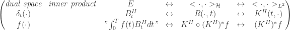
, ![K^H(t,s)=1_{[0,t]}(s),](https://s0.wp.com/latex.php?latex=K%5EH%28t%2Cs%29%3D1_%7B%5B0%2Ct%5D%7D%28s%29%2C+&bg=ffffff&fg=333333&s=0&c=20201002) , we can check
, we can check![E(B_tB_s)=<t\wedge\cdot, s\wedge\cdot>_{\mathcal{H}}=<1_{[0,t]}(\cdot),1_{[0,s]}(\cdot)>_{L^2}](https://s0.wp.com/latex.php?latex=E%28B_tB_s%29%3D%3Ct%5Cwedge%5Ccdot%2C+s%5Cwedge%5Ccdot%3E_%7B%5Cmathcal%7BH%7D%7D%3D%3C1_%7B%5B0%2Ct%5D%7D%28%5Ccdot%29%2C1_%7B%5B0%2Cs%5D%7D%28%5Ccdot%29%3E_%7BL%5E2%7D&bg=ffffff&fg=333333&s=0&c=20201002)
 uniquely defines a RKHS
  with the inner product
  is a Gaussian process satisfying

 , where
 ,
, ,
,
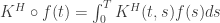
 where
where  is the Cholesky decomposition of
  , i.e (
 )
)

 where
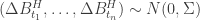
where  , now if we generate
  ,
, , then
 ![X_1[1:n]\sim N(0,\Sigma)](https://s0.wp.com/latex.php?latex=X_1%5B1%3An%5D%5Csim+N%280%2C%5CSigma%29&bg=ffffff&fg=333333&s=0&c=20201002) and
and ![X_2[1:n]\sim N(0,\Sigma)](https://s0.wp.com/latex.php?latex=X_2%5B1%3An%5D%5Csim+N%280%2C%5CSigma%29&bg=ffffff&fg=333333&s=0&c=20201002)
 and thus
 ? The property of circulant matrix shows that
 , i.e
, i.e that can be achieved by FFT.
 will be
